#tidytuesday: tour de france winners 🚴
Apr 7, 2020 00:00 · 2163 words · 11 minute read
For this week’s #TidyTuesday, I decided that I wanted to do an in-depth exploration of the this week’s dataset of Tour de France winners, and write a blog post about how I generally go about my data exploration for Tidy Tuesday.
However, I desperately need to preface this blog post: I went into this week’s #TidyTuesday excited to learn more about a sport I know almost nothing about. I’ve come out of it completely obsessed with the drama and insanity that is the history of the Tour de France.
I’m serious. If you know nothing about the Tour de France (like me, and probably most people), please go take a look at the Tour de France wikipedia page. I will be peppering in some of my favourite facts that I learned about the race and its history throughout this blog post but here are some of the best (in my opinion):
- The Tour de France originated as a publicity stunt for a failing sports newspaper (L’Auto) in France
- Apparently, setting up bike races to promote newspaper sales was a common thing in France at the time. No I am not kidding.
- L’Auto was actually a rival newspaper of the most popular sport paper in France at the time: Le Vélo. L’Auto hoped that this crazy long bike race might put Le Vélo out of business.
- The reason they were rivals? A disagreement over whether or not an infamous French officer sold military secrets to the Germans. (Was that not your first guess?)
- Competing in the Tour de France during its origins was crazy dangerous. Not only did the riders cycle on dirt roads with single-gear bikes, the race was almost cancelled after its first year because fans were constantly assaulting cyclists to give their favourite the lead.
So there’s your useless trivia for the week. I kind of wish this was a whole blog post about just how crazy the Tour de France is but the context makes the data as a whole more fun too.
Data Exploration
Just a quick heads up: the full code for this week’s #TidyTuesday can be found on my github.
First things first, we have to load some useful packages, get the data, and see what it looks like.
# Load libraries
library(tidyverse)    # All the fun tidy functions!
library(skimr)        # Gives an awesome data summary for exploration
library(lubridate)    # For working with dates

# Read data
tdf_winners <- read_csv('https://raw.githubusercontent.com/rfordatascience/tidytuesday/master/data/2020/2020-04-07/tdf_winners.csv')
tdf_winners
## # A tibble: 106 x 19
## edition start_date winner_name winner_team distance time_overall time_margin
## <dbl> <date> <chr> <chr> <dbl> <dbl> <dbl>
## 1 1 1903-07-01 Maurice Ga~ La Françai~ 2428 94.6 2.99
## 2 2 1904-07-02 Henri Corn~ Conte 2428 96.1 2.27
## 3 3 1905-07-09 Louis Trou~ Peugeot–Wo~ 2994 NA NA
## 4 4 1906-07-04 René Potti~ Peugeot–Wo~ 4637 NA NA
## 5 5 1907-07-08 Lucien Pet~ Peugeot–Wo~ 4488 NA NA
## 6 6 1908-07-13 Lucien Pet~ Peugeot–Wo~ 4497 NA NA
## 7 7 1909-07-05 François F~ Alcyon–Dun~ 4498 NA NA
## 8 8 1910-07-01 Octave Lap~ Alcyon–Dun~ 4734 NA NA
## 9 9 1911-07-02 Gustave Ga~ Alcyon–Dun~ 5343 NA NA
## 10 10 1912-06-30 Odile Defr~ Alcyon–Dun~ 5289 NA NA
## # ... with 96 more rows, and 12 more variables: stage_wins <dbl>,
## # stages_led <dbl>, height <dbl>, weight <dbl>, age <dbl>, born <date>,
## # died <date>, full_name <chr>, nickname <chr>, birth_town <chr>,
## # birth_country <chr>, nationality <chr>When I’m exploring data, sometimes I have a really hard time knowing where to start. My favourite thing to do is start at the same spot everytime and just do a simple glimpse and skim of the data.
glimpse(tdf_winners)## Observations: 106
## Variables: 19
## $ edition <dbl> 1, 2, 3, 4, 5, 6, 7, 8, 9, 10, 11, 12, 13, 14, 15, 16...
## $ start_date <date> 1903-07-01, 1904-07-02, 1905-07-09, 1906-07-04, 1907...
## $ winner_name <chr> "Maurice Garin", "Henri Cornet", "Louis Trousselier",...
## $ winner_team <chr> "La Française", "Conte", "Peugeot–Wolber", "Peugeot–W...
## $ distance <dbl> 2428, 2428, 2994, 4637, 4488, 4497, 4498, 4734, 5343,...
## $ time_overall <dbl> 94.55389, 96.09861, NA, NA, NA, NA, NA, NA, NA, NA, 1...
## $ time_margin <dbl> 2.98916667, 2.27055556, NA, NA, NA, NA, NA, NA, NA, N...
## $ stage_wins <dbl> 3, 1, 5, 5, 2, 5, 6, 4, 2, 3, 1, 1, 1, 4, 2, 0, 3, 4,...
## $ stages_led <dbl> 6, 3, 10, 12, 5, 13, 13, 3, 13, 13, 8, 15, 2, 14, 14,...
## $ height <dbl> 1.62, NA, NA, NA, NA, NA, 1.78, NA, NA, NA, NA, NA, N...
## $ weight <dbl> 60, NA, NA, NA, NA, NA, 88, NA, NA, NA, NA, NA, NA, N...
## $ age <dbl> 32, 19, 24, 27, 24, 25, 22, 22, 26, 23, 23, 24, 33, 3...
## $ born <date> 1871-03-03, 1884-08-04, 1881-06-29, 1879-06-05, 1882...
## $ died <date> 1957-02-19, 1941-03-18, 1939-04-24, 1907-01-25, 1917...
## $ full_name <chr> NA, NA, NA, NA, "Lucien Georges Mazan", "Lucien Georg...
## $ nickname <chr> "The Little Chimney-sweep", "Le rigolo (The joker)", ...
## $ birth_town <chr> "Arvier", "Desvres", "Paris", "Moret-sur-Loing", "Ple...
## $ birth_country <chr> "Italy", "France", "France", "France", "France", "Fra...
## $ nationality <chr> " France", " France", " France", " France", " France"...In this glimpse we can see the dimensions and the general structure of the data. This is not a very big dataset: we have 106 rows (one row for each edition of the Tour de France) and 19 columns with various information about each Tour de France winner. We can start to see that there are quite a few NA values popping up in this glimpse. I assume this is because the Tour de France originated in 1903 and there’s likely no reliable record of the winners’ heights, weights, etc. So this is not too problematic in terms of the data’s trustworthiness.
skim(tdf_winners)| Name | tdf_winners |
| Number of rows | 106 |
| Number of columns | 19 |
| _______________________ | |
| Column type frequency: | |
| character | 7 |
| Date | 3 |
| numeric | 9 |
| ________________________ | |
| Group variables | None |
Variable type: character
| skim_variable | n_missing | complete_rate | min | max | empty | n_unique | whitespace |
|---|---|---|---|---|---|---|---|
| winner_name | 0 | 1.00 | 10 | 19 | 0 | 63 | 0 |
| winner_team | 0 | 1.00 | 3 | 33 | 0 | 48 | 0 |
| full_name | 60 | 0.43 | 15 | 33 | 0 | 23 | 0 |
| nickname | 32 | 0.70 | 1 | 95 | 0 | 37 | 0 |
| birth_town | 0 | 1.00 | 3 | 28 | 0 | 58 | 0 |
| birth_country | 0 | 1.00 | 3 | 11 | 0 | 15 | 0 |
| nationality | 0 | 1.00 | 6 | 14 | 0 | 14 | 106 |
Variable type: Date
| skim_variable | n_missing | complete_rate | min | max | median | n_unique |
|---|---|---|---|---|---|---|
| start_date | 0 | 1.00 | 1903-07-01 | 2019-07-06 | 1966-12-24 | 106 |
| born | 0 | 1.00 | 1871-03-03 | 1997-01-13 | 1940-12-27 | 63 |
| died | 50 | 0.53 | 1907-01-25 | 2019-08-16 | 1980-04-10 | 38 |
Variable type: numeric
| skim_variable | n_missing | complete_rate | mean | sd | p0 | p25 | p50 | p75 | p100 | hist |
|---|---|---|---|---|---|---|---|---|---|---|
| edition | 0 | 1.00 | 53.50 | 30.74 | 1.00 | 27.25 | 53.50 | 79.75 | 106.00 | ▇▇▇▇▇ |
| distance | 0 | 1.00 | 4212.06 | 704.28 | 2428.00 | 3657.88 | 4155.50 | 4652.50 | 5745.00 | ▁▇▇▆▃ |
| time_overall | 8 | 0.92 | 125.75 | 41.56 | 82.09 | 92.60 | 115.03 | 142.68 | 238.74 | ▇▅▂▁▂ |
| time_margin | 8 | 0.92 | 0.27 | 0.48 | 0.00 | 0.05 | 0.10 | 0.25 | 2.99 | ▇▁▁▁▁ |
| stage_wins | 0 | 1.00 | 2.74 | 1.84 | 0.00 | 1.00 | 2.00 | 4.00 | 8.00 | ▆▇▃▂▁ |
| stages_led | 0 | 1.00 | 10.79 | 5.31 | 1.00 | 6.25 | 12.00 | 14.00 | 22.00 | ▆▇▇▇▃ |
| height | 40 | 0.62 | 1.78 | 0.06 | 1.61 | 1.74 | 1.77 | 1.82 | 1.90 | ▁▁▇▃▂ |
| weight | 39 | 0.63 | 69.25 | 6.59 | 52.00 | 64.50 | 69.00 | 74.00 | 88.00 | ▁▆▇▇▁ |
| age | 0 | 1.00 | 27.72 | 3.35 | 19.00 | 26.00 | 28.00 | 30.00 | 36.00 | ▁▃▇▃▂ |
I found skim to be super helpful (and interesting) for this particular dataset, giving us lots of ideas for things that we can explore further.
Some things that I noticed from looking at the skim output:
- there’s been 106 Tour de France editions but only 63 unique individual winners
full_namehas more missing values thannickname- in 106 editions, there have only been winners from 14 unique nationalities
- the distance of the tour varies quite a bit. I know that the route is different from edition to edition but a range of 5000km seems dramatic.
This is a great starting point for exploration! Let’s dig into it a little more ⛏️.
Racers with multiple TDF wins
We noticed that there were only 63 unique values for the winner_name variable. That means that there must be cyclists who have won multiple Tour de France editions.
tdf_winners %>%
  count(winner_name, sort = TRUE) %>%
  filter(n > 1) %>%
  summarise(
    num_of_racers = n_distinct(winner_name),
    num_of_wins = sum(n)
    ) %>%
  kable() %>%
kable_styling()| num_of_racers | num_of_wins |
|---|---|
| 21 | 64 |
So half of the editions in all Tour de France history were won by just 21 cyclists! That’s a pretty cool. Who were these cyclists and how many times did they win individually?
tdf_winners %>%
  count(winner_name, name = 'num_of_wins') %>%
  filter(num_of_wins > 1) %>%
  ggplot(aes(reorder(winner_name, num_of_wins), num_of_wins)) +
  geom_col(fill = pal[1],
           width = 0.6,
           alpha = 0.8) +
  labs(x = NULL, y = 'Tour de France wins') +
  coord_flip()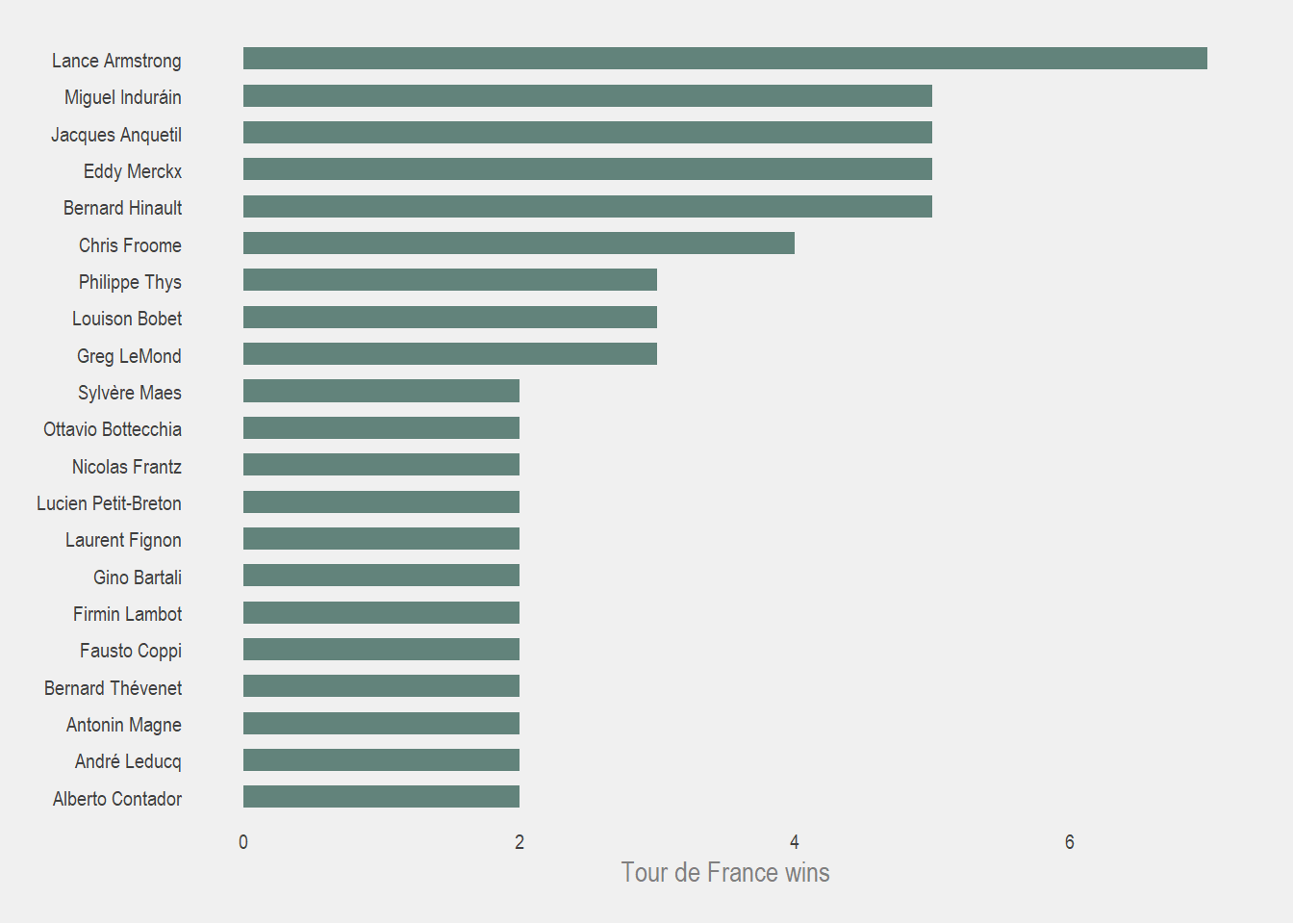
Personally, I am only familiar with the top guy (as I’m sure most people are), but it’s pretty cool to see just how many cyclists that were not just able to win this race once, but more than once. That’s an amazing feat of human strength and endurance (and drugs…? 👀).
In my wikipedia spiral, I learned that Eddy Merckx was a pretty big deal in the 70s. He was the first “superstar” of the Tour de France and his aggressive style earned him the nickname “The Cannibal”. (Side note: Cycling is way more intense than I ever could have imagined)
Nations that have a Tour de France winner
Another thing we noticed was that only 14 countries can claim competitors who have won an edition of the Tour de France.
tdf_winners %>%
  count(nationality, sort = TRUE) %>%
  ggplot(aes(reorder(nationality, n), n)) +
  geom_col(fill = pal[2], alpha = 0.8, width = 0.6) +
  labs(x = NULL, y = 'Tour de France wins') +
  coord_flip()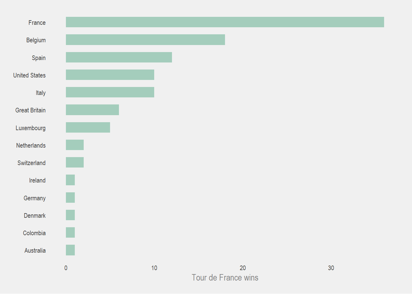
It’s not surprising that France has won so many editions of the Tour. The race originated there and although it was open for global competitors for most of its editions, it was the most popular in France (and neighbouring countries) for most of the 20th century. This meant that there were more cyclists who were racing from western European countries than anywhere else. In fact the only countries who have won outside of “Europe” (sorry Brexit) are: USA, Colombia, and Australia.
Race distances
We noticed before the huge variability of the race distances. To me, this didn’t make a lot of sense. I expected a bit of variability since the route changes from edition to edition but variance of the range of distances travelled over the years is very wide.
ggplot(tdf_winners, aes(distance)) +
  geom_histogram(fill = pal[3], binwidth = 200, alpha = 0.8) +
  labs(x = 'Race distance (km)', y = 'Frequency')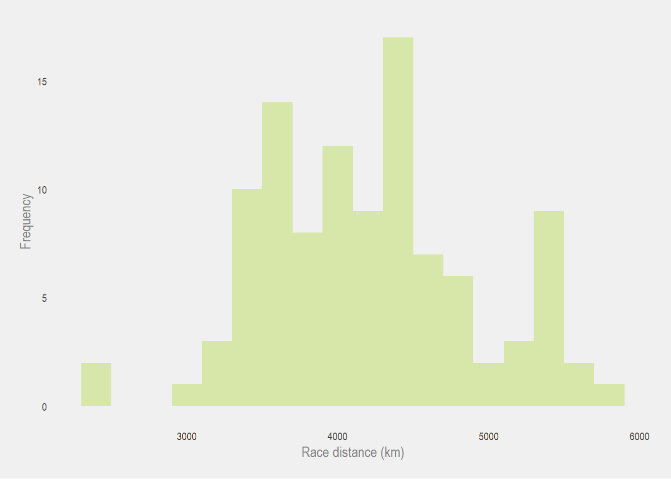
How can the race distance differ from low 3000s km to almost 6000km? After looking into the history, I decided to plot the distances raced over the years.
tdf_winners %>%
  mutate(start_year = year(start_date)) %>%
  ggplot(aes(start_year, distance)) +
  geom_line(col = pal[4]) +
  geom_point(data = min_max_dist,
             aes(start_year, distance),
             col = 'grey35') +
  geom_text(data = min_max_dist,
            aes(label = start_year),
            size = 3,
            color = 'grey25',
            hjust = -0.25,
            family = 'Arial Narrow') +
  labs(x = 'Race year', y = 'Race distance (km)')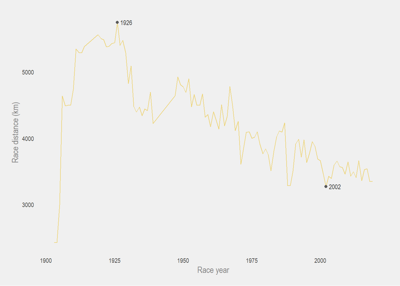
We can see that since the race’s origins, the race distance seems to be on a bit of a decline. Not considering the first year of the race in 1903, the minimum distance raced was 3272km (which is still crazy). The maximum distance raced clocks in at a whopping 5745km during the 1926 edition of the Tour (which is actual insanity???). If you’re wondering why the distances are so insanely high during the early 1900s, it lies (once again) within the history of the Tour de France.
The original organizer of the race was a strict traditionalist and wanted the race to be the ultimate test of endurance, stating that the ideal race had only ONE rider making it to the finish line (omg). He also demanded that riders mend their bicycles without help and that they use the same bicycle from start to end. Exchanging a damaged bicycle for another was not allowed under his rules (OMG).
So, in conclusion… The Tour de France is crazy.
Actually though, I haven’t even touched the doping scandals that have plagued the race since the 1960s or the fact that the race was never really standardized until the 80s or the fact that it remained a newspaper feud for 40 years after its origin. Everything about the race is wild.
This is an awesome #TidyTuesday dataset and there’s still so much more to explore past what I’ve looked at here. I think this dataset is a great example of how context (or domain expertise as it’s called in the data science world) is pretty important to understanding your data (and a great illustration of the joy of learning new things).
Any question/comments/fun facts about the Tour de France can be directed to my twitter. Reminder that you can find my full code for this week’s Tidy Tuesday on github. Happy #TidyTuesday everyone! ☺